Building critical thinking infrastructure

A companion to When Deliberation Meets Reality, which argued that the missing precondition for collective flourishing is critical thinking infrastructure fast enough to survive contact with reality. This post, Part 2 of the Critical thinking infrastructure essay series, describes what that infrastructure looks like.

Abstract

This post proposes what decision-support infrastructure must look like to compress time-to-question and time-to-answer enough to fit rigorous analysis inside the decision window. It describes a four-layer architecture (spatial knowledge graph, domain graph, solver integration, micro-tools) governed by nine principles. Three matter most here: separating stable spatial knowledge from volatile project data, keeping logic out of data objects, and treating materialisation as an economic decision rather than a structural one. The architecture draws on six years of commercial deployment in logistics planning. The post is a ledger: what has been tested, what has been designed, what remains an open research question.

Hypotheses introduced (one per section):

1. Asking a strategic question about a physical system is dominated by a cascade of bottlenecks. They begin with the absence of a shared domain model and end with questions that are never discovered.
2. Three interventions break the cascade: formalise the domain model, pre-build the stable spatial foundation, design the analytical layer for composability. Each addresses a different bottleneck. They reinforce each other.
3. Once the cascade is broken, the explore-decide cycle compresses from weeks to minutes. Decision quality then turns on the decision-maker’s ability to ask good questions, which itself improves with each iteration.
4. Once a deployment is running, the binding constraint on ttQ is translating a decision-maker’s natural-language question into the system’s formal query language. A human facilitator fills this role today. An AI facilitator can compress it further.
5. The bridge from individual decision support to collective flourishing is the inspectable trace. Fast, grounded decisions leave behind evidence the collective can challenge.
6. The honest assessment of any research programme is the ratio of tested claims to untested ones.

Introduction

The previous post proposed a hypothesis: analytically superior methods are abandoned under pressure, despite their rigour, because they are too slow to fit inside the window where decisions get made. If that hypothesis holds, the binding constraint on decision quality is time, not analytical sophistication. Specifically, the time it takes to formulate a question (ttQ) and receive a useful answer (ttA). When those times are large, decision-makers default to gut feel regardless of what tools are available. When they shrink enough to permit rapid iteration, decisions improve, because each answer opens a better question than the last.

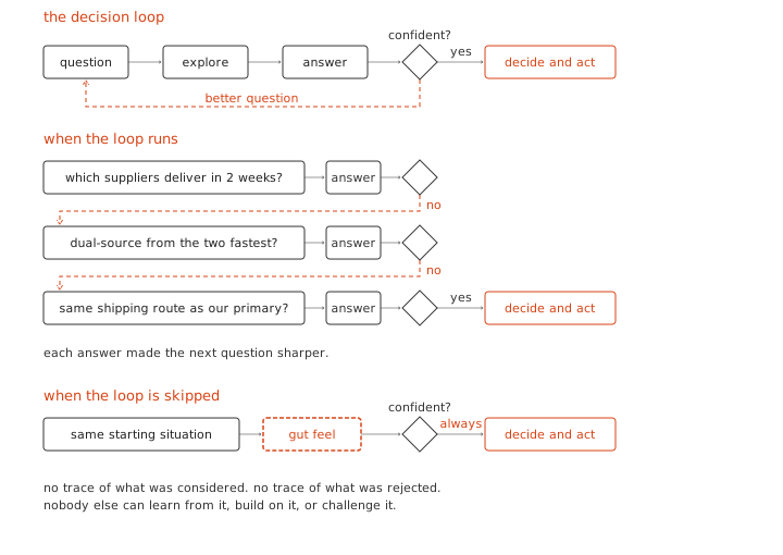
This post offers a constructive proposal. What would a system look like that compresses ttQ and ttA to the point where rigorous analysis fits inside the decision window?

The architecture has been developed through a mix of commercial deployment and design research. It builds on logistics planning platforms used on operational decisions worth hundreds of millions of dollars. Different versions have been running in production since 2020; earlier versions date to 2016. What follows describes what works, what remains to be built, and where the research questions are.

Where the time actually goes

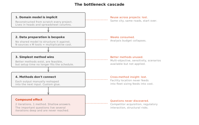
Hypothesis: asking a strategic question about a physical system is dominated by a cascade of bottlenecks. They begin with the absence of a shared domain model and end with questions that are never discovered.

Consider a logistics company deciding whether to bid on a government contract worth hundreds of millions over five years. The questions that decide the outcome are strategic. Can we service this geography profitably given our existing infrastructure? Where are the gaps between what we currently operate and what the tender requires? Three competitors went into administration last year; should we acquire their contracts, and which? The government is introducing low-emission zones next year; what percentage of our operations fall inside them, and what does compliance cost us?

Each question has a quantitative answer that depends on spatial data: the geography, the road network, the building stock, the regulatory boundaries, the locations of existing infrastructure. The analytical methods exist, and many are cheap to run on modern hardware. The problem is everything that sits between the question and the method.

The first bottleneck is the domain model. Every project carries an implicit ontology: what counts as a “service point”, how “coverage” is defined, what “profitability” means in terms of cost components, how the client’s operational categories map onto geographic and regulatory boundaries. This domain knowledge is rarely formalised. It lives in tender documents, in the heads of experienced planners, in the column names of spreadsheets, in the assumptions buried inside previous analyses. It gets reconstructed from scratch on every project, which is why data from one engagement cannot be reused on the next even when both operate in the same city.

The second bottleneck is data preparation. Geocoding thousands of addresses, computing distances across the road network, cleaning and spatially locating property data, mapping administrative and regulatory boundaries, matching the client’s data against authoritative sources. This work repeats across projects, but because there is no shared domain model to structure it against, each transformation is bespoke.

The third bottleneck is method selection. With most of the timeline consumed by the first two, the team reaches for the simplest analytical method that can produce a defensible answer in the time left. Multi-objective optimisation, spatial sensitivity analysis, scenario comparison across parameter ranges, are all computationally feasible. Each requires its own setup, calibration, and interpretation time that the schedule no longer permits.

The fourth bottleneck is integration between methods. Feeding the output of a facility location model into a fleet sizing calculation and then into a cost projection requires custom glue at each step. Without a shared data layer, each method’s output has to be reshaped by hand into the next method’s input.

These bottlenecks compound. A four-week tender timeline might produce two iterations of the explore-decide cycle using a single method. The plan is defensible, because two good answers were produced. It is also shallow, because the methods that would have revealed trade-offs, risks, and structural weaknesses were never applied. The deepest cost is in the questions that are never asked. The question about acquiring a competitor’s contracts is never formulated, because you only discover it after several iterations of analysing the competitive landscape, and the bottlenecks prevent you from getting that far. The important questions live several iterations deep, and the cascade of setup costs keeps you from reaching them.

The architectural response

Hypothesis: three interventions break the cascade: formalise the domain model, pre-build the stable spatial foundation, design the analytical layer for composability. Each addresses a different bottleneck. They reinforce each other.

The architecture responds at four levels.

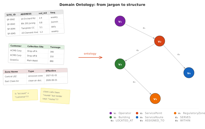
The first response makes the domain model explicit. Every planning problem carries an implicit ontology: what entity types exist (buildings, roads, service points, vehicles, regulatory zones), what relationships matter between them, and what vocabulary the domain uses to describe its questions. In the traditional workflow, this ontology is never written down. It is reconstructed through conversation with the client, through inspection of their spreadsheets, and through the analyst’s prior experience. The architecture externalises this as a declarative domain ontology: a configuration file, loaded at runtime, that defines the node types, edge types, and relationships meaningful to a given deployment¹. A Singapore logistics engagement loads one ontology. A UK waste management engagement loads another. The graph engine underneath is domain-agnostic and does not change. When the domain model is explicit, data from one project structured against that ontology becomes reusable on the next.

The second response separates what is stable from what varies. Logistics problems, urban planning problems, facility location problems, and supply chain distribution problems all operate on the same physical substrate. Roads, buildings, administrative boundaries, points of interest: these exist independently of any planning question, change over months or years, and are shared across every project in the same geography. What varies between projects is the operational question: which properties to service, what infrastructure to deploy, how to schedule operations. The architecture separates these into layers with different rates of change².

Layer 1: The Spatial Knowledge Graph.

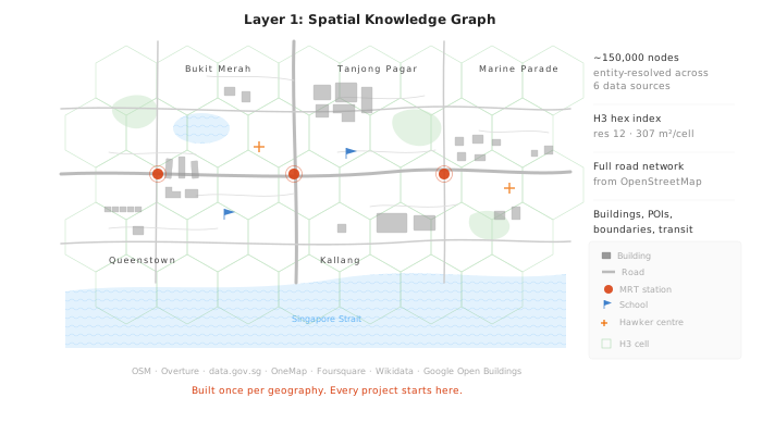
The stable foundation. It captures the physical reality of a geography by fusing data from government registries, commercial databases, crowdsourced mapping platforms, satellite-derived building footprints, and structured knowledge bases. For a city like Singapore, that means around 100,000 to 150,000 unique real-world entities, spatially indexed using a hexagonal hierarchical system (H3), with cross-links resolved through entity resolution³. Built once per geography, structured against the domain ontology, shared across all projects.

Layer 2: The Domain Graph.

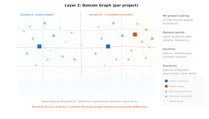
The operational problem: demand points, facilities, constraints, decision scenarios. Specific to each project. Parameterised against the spatial knowledge graph and the loaded ontology rather than built from scratch. A new project inherits the full spatial foundation and the full domain vocabulary, and adds only the operational specifics.

The third response addresses the integration bottleneck.

Layer 3: Solver Integration.

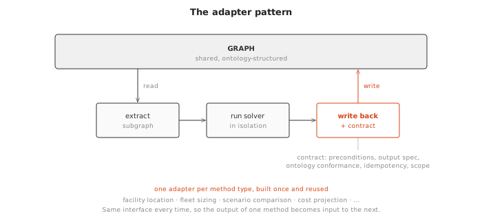
Analytical methods (optimisation, location modelling, fleet sizing, scenario comparison) run through disciplined adapter pipelines that isolate each method from the graph and from each other. Each adapter follows a three-step pattern: extract the relevant subgraph into the method’s expected input format, run the method in isolation, write the results back through a formal contract⁴. The contract is what makes methods composable: the output of a facility location model can feed into a fleet sizing calculation because both read from and write to the same graph through the same interface. A new adapter is built once per method type and reused across all projects that need it.

The fourth response addresses method accessibility.

Layer 4: Micro-tools.

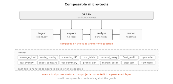
Small, composable, read-only tools that handle work specific to a particular question: ingesting a client’s data file, exploring a spatial pattern interactively, running a sensitivity analysis on a parameter, rendering results in a particular format. Micro-tools are cheap to build, typically minutes to hours. They compose freely with each other and with the solver layer. The cost of trying an additional analytical method drops from days of custom integration work to the time it takes to compose a new micro-tool against the existing graph. When a micro-tool proves useful across many projects, that reuse is the signal to promote it to a more permanent layer⁵.

One useful side effect: the micro-tools layer is itself a decent way to set up the domain ontology layer and link it to the Spatial Knowledge Graph.

The economic consequence of this separation is that the second project in a geography costs a fraction of the first, and the tenth costs almost nothing to set up. The deeper consequence is what the team does with the time the cascade used to consume. The domain model is already formalised. The spatial foundation is already built. Methods connect through shared interfaces rather than custom glue. Trying an additional analytical approach is cheap. What remains is the work that requires human expertise: asking the right questions and interpreting the answers.

What this means for question-answer speed

Hypothesis: once the cascade is broken, the explore-decide cycle compresses from weeks to minutes. Decision quality then turns on the decision-maker’s ability to ask good questions, which itself improves with each iteration.

With the spatial foundation pre-built and the domain ontology loaded, each question traces a path through the architecture in minutes rather than weeks. An example:

Iteration 1: “Can we profitably service the eastern districts given our current depot locations?”

• Domain Ontology: defines what “service profitability” means for this domain: cost components, coverage thresholds, demand metrics
• Layer 1 (Spatial KG): eastern district boundaries are already resolved as H3 cell sets; building stock, road distances, and population proxies are pre-indexed
• Layer 2 (Domain Graph): current depot locations and demand points loaded as the project overlay
• Layer 3 (Solver Integration): coverage model computes service reach per depot; cost projection estimates margin
• Layer 4 (Micro-tools): spatial filter (restrict to eastern planning areas), coverage heatmap, cost summary table

Answer in four minutes: eastern districts viable at 12% margin, but three uncovered zones near industrial parks. That answer reveals the next question.

Iteration 2: “What if the competitor’s eastern contracts become available?”

• Domain Ontology: same schema; “competitor contract” maps to a set of additional demand points with volume history
• Layer 1 (Spatial KG): unchanged, already loaded
• Layer 2 (Domain Graph): scenario overlay adds the competitor’s service area as new demand nodes linked to the same spatial foundation; the base scenario is untouched
• Layer 3 (Solver Integration): re-runs coverage and cost with the additional demand volume
• Layer 4 (Micro-tools): scenario comparison (side-by-side delta between Scenario A and Scenario B), volume impact summary

Answer in three minutes: margin improves to 18% with the added volume, but 40% of the new service area falls inside the proposed low-emission zone. That overlap prompts the next question.

Iteration 3: “How does the LEZ interact with our fleet age?”

• Domain Ontology: RegulatoryZone and Fleet node types linked through compliance edges; the ontology defines what “compliant” means for each zone type and emission class
• Layer 1 (Spatial KG): LEZ boundary polygons are already in the graph as RegulatoryZone nodes, spatially indexed and linked to buildings via WITHIN edges
• Layer 2 (Domain Graph): fleet asset records with age and emission class; routes from the previous solver run
• Layer 3 (Solver Integration): compliance checker cross-references active routes against zone requirements per vehicle
• Layer 4 (Micro-tools): spatial overlay (fleet routes × LEZ boundaries), compliance gap report, fleet renewal cost estimator

Answer in five minutes: the real constraint is regulatory, not operational. Fleet renewal cost to achieve LEZ compliance exceeds the margin gain from the competitor acquisition. The bid strategy changes.

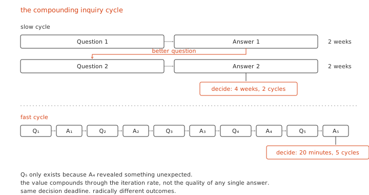
Three iterations in twelve minutes, each building on the last. The traditional workflow would have produced one of these answers in four weeks, and the third question would never have been asked, because it only exists as a consequence of the second answer.

This is the compounding inquiry cycle from the previous post. Value lives in the iteration rate, and the iteration rate is set by time-to-answer. When ttA drops from days to minutes, the number of iterations in a fixed window rises by orders of magnitude, and each iteration produces a better question than the last.

The facilitator: from human to AI

Hypothesis: once a deployment is running, the binding constraint on ttQ is translating a decision-maker’s natural-language question into the system’s formal query language. A human facilitator fills this role today. An AI facilitator can compress it further.

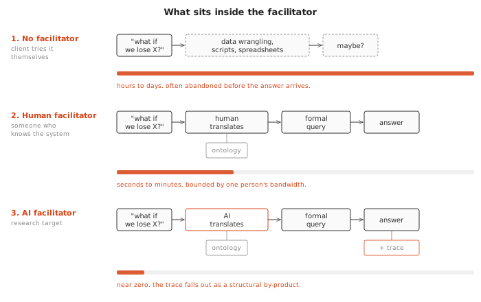
The example above assumed somebody was driving the system. In the commercial deployments that preceded this architecture, I was the human facilitator (or, by the latest obfuscation, an AI forward deployment engineer). The client would ask in natural language: “What happens if we lose that depot?” I would translate that into parameters and some custom code, run the scenario, present the results, and take the follow-up. We could run five or ten iterations in a session. The previous workflow, where the client’s team performed the same analysis internally, took about two weeks per iteration.

The facilitator role is where the real compression happens. The client’s ttQ is instantaneous for them. They are the experts and the decision-makers. Answers lead quickly to higher-order questions. The conversation among the decision-makers becomes deep enough that they forget you are in the room, right up until they ask for something the system cannot quickly run. The delay sits in translation: converting their question into something the system can execute. With a human facilitator who knows the system (and the system set up as above), translation takes seconds. Without one, it takes the client hours or days of data wrangling, if they attempt it at all.

The research question is whether an AI can perform this translation. Large language models already convert natural language into structured queries. The specific challenge here is that the translation requires domain knowledge: understanding what the client means by “lose that depot” in the context of the loaded spatial graph, the active scenario, and the constraints of the current problem. That domain knowledge lives in the ontology¹, the graph schema that defines what node and edge types are meaningful for a given deployment.

If the AI facilitator works, ttQ drops to near zero for the decision-maker. They ask in natural language, the AI translates against the loaded ontology, the system executes, and the answer comes back with the full reasoning trace attached. The decision-maker’s domain expertise, their ability to formulate the right question at the right moment, becomes the scarce resource the platform amplifies.

This is where the inspectability argument from the previous post becomes architectural rather than aspirational. Every question the AI facilitator translates produces a formal query against the graph. Every answer traces back to specific nodes, edges, and solver outputs. The reasoning trace is a structural consequence of how the system works.

Connecting back: from individual decisions to collective flourishing

Hypothesis: the bridge from individual decision support to collective flourishing is the inspectable trace. Fast, grounded decisions leave behind evidence the collective can challenge.

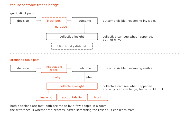
Wheeler’s vision is about societies seeing, reasoning, and choosing together. The architecture described here makes individual and small-group decisions fast and inspectable, so the collective can engage with the reasoning after the fact.

Consider a government making a supply chain decision under crisis pressure. The system lets three people in a room explore scenarios, compare trade-offs, and choose a course of action in minutes. After the decision, the trace remains: what was asked, what data was queried, what alternatives were considered, what was chosen and why. Regulators, affected communities, and accountability mechanisms can engage with that trace and ask “why was the cheaper but riskier supplier chosen?” and receive an answer grounded in the actual scenario comparison rather than a post-hoc narrative.

This is a different model of collective flourishing than distributed deliberation. It accepts that decisions may be fast and narrow, and asks only that those decisions leave behind reasoning the collective can inspect, challenge, and learn from.

Whether this works is an empirical question. The hypothesis register that accompanies this series identifies fourteen testable claims, seven open questions for self-critique, and explicit conditions under which the thesis would be falsified⁶.

The next posts in the series extend the argument: why no single model will save us, and what it takes to turn this from a platform into public infrastructure.

What remains to be built, and what remains to be proven

Hypothesis: the honest assessment of any research programme is the ratio of tested claims to untested ones.

Tested through commercial deployment (2020 onwards):

• The explore-decide cycle produces measurably better plans than the traditional workflow. Clients who used a bespoke version of the system with a human facilitator explored more scenarios and produced tighter bids.
• The human facilitator role is critical. Without a facilitator translating between the decision-maker and the system, the decision-maker reverts to familiar tools.
• Scenario comparison changes how decision-makers think. Once they see alternatives side by side, they ask different and better questions.

These deployments ran on bespoke, project-specific implementations rather than the knowledge graph architecture described in this post. The graph itself is only being tested in 2026.

Designed conceptually (2026):

• The four-layer architecture with nine governing principles (P1 through P9).
• The domain ontology framework that allows the same engine to serve different problem domains through configuration rather than code changes.
• The solver integration pipeline (extract-solve-rehydrate) with formal contracts.
• The Rust implementation, chosen for memory safety, predictable performance, and strong geospatial ecosystem fit.

Open research questions:

• The AI facilitator. Can an LLM reliably translate natural-language questions into graph queries against a loaded domain ontology? What is the error rate, and what does graceful degradation look like when the translation is wrong?
• Multi-organisation data sharing. Can the architecture produce useful results with partial data, where each organisation contributes what it is willing to share without revealing competitive information?
• Collective inspectability at scale. Do inspectable decision traces actually get inspected? By whom? Under what conditions?
• The speed benchmark against ungrounded AI. Can grounded, knowledge-graph-backed answers match the speed of raw LLM responses while keeping traceability? If they are slightly slower, does traceability make up the difference, or does speed always win?

The last question is the most consequential, and the most uncomfortable. The previous post argued that speed is the binding constraint. If that is true, then any system that adds grounding at the cost of speed will lose to one that does not. The bet is that grounding and speed are not fundamentally in tension; that a well-designed knowledge graph with an effective AI facilitator can deliver both. That bet needs to be tested, not assumed.